02_iSEE.Rmd

# Interactive SummarizedExperiment visualizations

Instructor: Melissa Mayén Quiroz


> How can you make plots from "SummarizedExperiment" objects without having to write any code? 
>
> The answer is with "iSEE"

* http://bioconductor.org/packages/iSEE
* http://bioconductor.org/packages/release/bioc/vignettes/iSEE/inst/doc/basic.html


`iSEE` is a Bioconductor package that provides an interactive Shiny-based graphical user interface for exploring data stored in `SummarizedExperiment` objects (Rue-Albrecht et al. 2018). 


## Classes for iSEE

`SummarizedExperiment` (SE) and `SingleCellExperiment` (SCE) are classes in R. Classes serve as templates for creating objects that contain data and methods for manipulating those data.

### SummarizedExperiment class

- Assay Data: The primary data matrix containing quantitative measurements, such as gene expression values or read counts. Rows represent features (e.g., genes, transcripts) and columns represent samples (e.g., experimental conditions, individuals).

- Row Metadata (`rowData`): Additional information about the features in the assay data. This can include annotations, identifiers, genomic coordinates, and other relevant information.

- Column Metadata (`colData`): Additional information about the samples in the assay data. This can include sample annotations, experimental conditions, treatment groups, and other relevant information.

- `metadata`: Additional information about the experiment.

### SingleCellExperiment

This object is specifically designed to store and analyze single-cell RNA sequencing (scRNA-seq) data. It extends the `SummarizedExperiment` class to include specialized features for single-cell data, such as cell identifiers, dimensionality reduction results, and methods for quality control and normalization.

- Assay Data: The primary data matrix containing gene expression values or other measurements. Rows represent genes and columns represent cells.

- `colData` (Column Metadata): Additional information about each cell, such as cell type, experimental condition, or any other relevant metadata.

- `rowData` (Row Metadata): Additional information about each gene, such as gene symbols, genomic coordinates, or functional annotations.

- `reducedDims`: Dimensionality reduction results, such as "principal component analysis" (PCA), "t-distributed stochastic neighbor embedding" (t-SNE), and 
"Uniform Manifold Approximation and Projection" (UMAP), used for visualizing and clustering cells.

- `altExpNames` and `altExps`: Names of alternative experiments (such as spike-in control genes used for normalization) and alternative experiment counts matrices.

- `metadata`: Additional metadata about the experiment.

### SpatialExperiment

This object extends the `SingleCellExperiment` class and is designed to store and analyze spatially-resolved transcriptomics data. Spatial transcriptomics combines gene expression data with spatial information, providing insights into the spatial organization of tissues.

- Assay Data: The primary data matrix containing gene expression values or other measurements. Rows represent genes and columns represent spatial spots or pixels.

- `colData` (Column Metadata): Additional information about each spatial spot or pixel, such as spatial coordinates, tissue section, or any other relevant metadata.

- `rowData` (Row Metadata): Additional information about each gene, such as gene symbols, genomic coordinates, or functional annotations.

- `spatialCoords`: A matrix or data frame containing the spatial coordinates (e.g., x and y coordinates) of each spot or pixel, which is crucial for spatial analyses and visualization.

- `imgData`: Links to image data associated with the spatial transcriptomics experiment, such as histology images or microscopy images, which provide the spatial context for the transcriptomics data.

- `reducedDims`: Dimensionality reduction results for visualizing and clustering spatial spots or pixels, similar to the SingleCellExperiment class.

- `metadata`: Additional metadata about the experiment.


## Getting Started with iSEE

[Reference manual](chrome-extension://efaidnbmnnnibpcajpcglclefindmkaj/https://bioconductor.org/packages/3.19/bioc/manuals/iSEE/man/iSEE.pdf)

Adapted from [The iSEE User's Guide](https://www.bioconductor.org/packages/release/bioc/vignettes/iSEE/inst/doc/basic.html)

- Installation (R version "4.4"). In this case, the package is already installed so we just need to load it.

```{r, load_iSEE}
# if (!require("BiocManager", quietly = TRUE))
#     install.packages("BiocManager")
#
# BiocManager::install("iSEE")

packageVersion("iSEE")
library("iSEE")
```

- Documentation

```{r, vignettes_iSEE, eval=FALSE}
browseVignettes("iSEE")
```

- Use (simple launch): 

If you have a `SummarizedExperiment` object (`se`) or an instance of a subclass, like a `SingleCellExperiment` object (sce), you can launch an `iSEE` app by running:

```{r, quick_launch, eval=interactive()}
## Launch iSEE for the se ("SummarizedExperiment" object)
iSEE(se)

## Launch iSEE for the sce ("SingleCellExperiment" object)
iSEE(sce)
```


## Description of the user interface 

![](https://raw.githubusercontent.com/lcolladotor/cshl_rstats_genome_scale_2024/devel/Figures/iSEE.png)

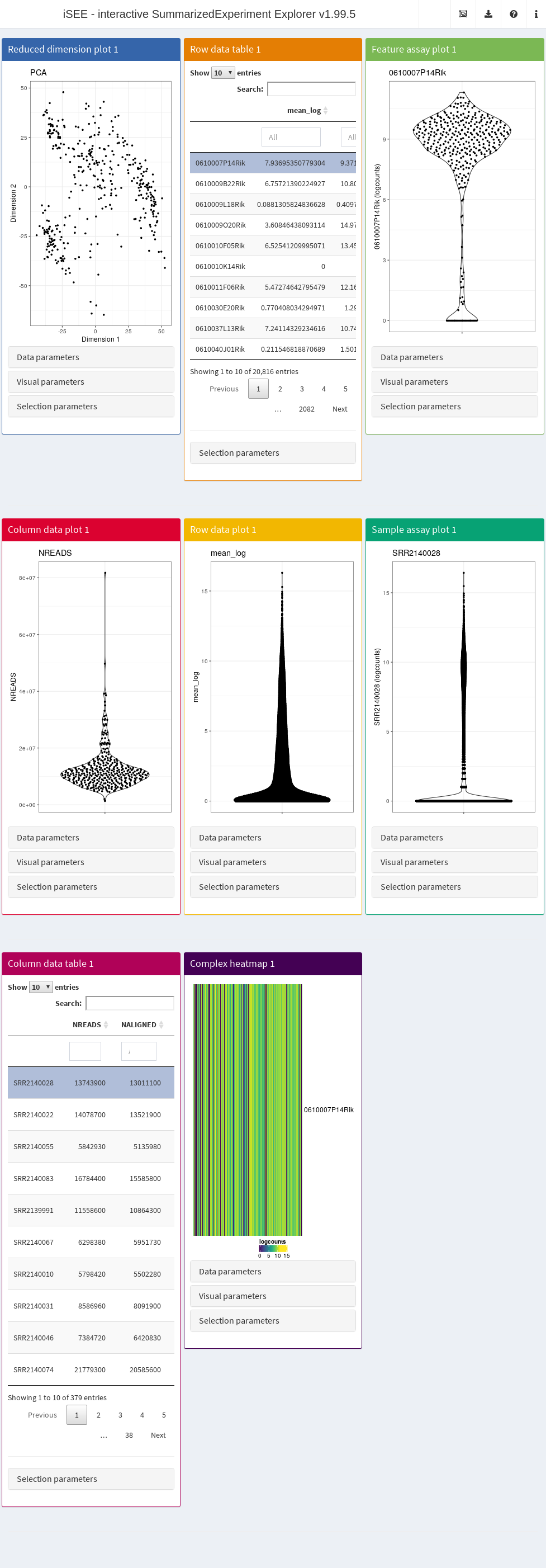
By default, the app starts with a dashboard that contains one panel or table of each type. By opening the collapsible panels named “Data parameters”, “Visual parameters”, and “Selection parameters” under each plot, we can control the content and appearance of each panel.

<div style="background-color:#E0EEE0; padding:20px; font-family: sans-serif">

Introductory tour:

In the upper right corner there is a question mark icon ❓. Clicking it and then on the hand button you can have an introductory tour. During this tour, you will be taken through the different components of the `iSEE` user interface and learn the basic usage mechanisms by doing small actions guided by the tutorial: the highlighted elements will be responding to your actions, while the rest of the UI will be shaded. 

</div>

### Header

The layout of the `iSEE` user interface uses the `shinydashboard` package. The dashboard header contains four dropdown menus.

- The “Organization” menu, which is identified by an icon displaying multiple windows
- “Export” dropdown menu, which is identified by a download icon
- The “Documentation” dropdown menu which is identified by a question mark icon ❓
- The “Additional Information” dropdown menu which is identified by the information icon ℹ️

#### Organization menu

The "Organization" dropdown menu, dentified by an icon displaying multiple windows, includes:

- "Organize panels” button opens a modal window that contains:
    - A selectize input to add, remove, and reorder panels in the main interface.
    - Two inputs to control the width and height, respectively, of each panel selected above. 

- The "Examine panel chart" feature, identified by a chain icon, allows you to visualize the relationships and point selections among your visible plot and table panels. Each panel is represented by a node, color-coded to match the app. (This functionality is particularly useful in sessions with many panels, helping you to see the structure of how panels send and receive data point selections).

<div style="background-color:#E0EEE0; padding:20px; font-family: sans-serif">

#### Export dropdown menu

The "Export” dropdown menu, identified by a download icon, includes:

- The "Download panel output" feature that allows you to download a zip folder containing the currently displayed panel content, including high-resolution figures and table contents as CSV files.

- The "Extract the R code" feature which provides a way to record the exact code that reproduces the current state of each plot. Clicking on this button opens a popup window with a text editor displaying the formatted code with syntax highlighting. You can copy this code, including initial lines and sessionInfo() commands, to your clipboard for inclusion in your analysis report or script. This code can then be further edited for publication.

- "Display panel settings" lets you export the code defining the current state of the panels in the interface. This is useful for pre-configuring an iSEE instance to start in the current state rather than with the default set of panels.

</div>

#### Documentation Menu

The "Documentation" dropdown, accessible through the question mark icon ❓, includes:

- Interactive Tour: Launches a guided tour of `iSEE`, teaching basic usage interactively.

- Open Vignette: Displays the iSEE vignette, either locally or from the Bioconductor project site.

#### Additional Information Menu

The "Additional Information" dropdown, accessible through the information icon ℹ️, includes:

- About this Session: Shows the output of the `sessionInfo()` function in a popup.
- About iSEE: Provides information on the development team, licensing, citation, and links to the GitHub repository for following development and contributing suggestions.


### Panel types

The main element in the body of iSEE is the combination of panels, generated (and optionally linked to one another) according to your actions. There are currently eight standard panel types that can be generated with iSEE:

- Reduced dimension plot
- Column data table
- Column data plot
- Feature assay plot
- Row data table
- Row data plot
- Sample assay plot
- Complex heatmap

In addition, custom panel types can be defined.

### Parameter sets

For each standard plot panel, three different sets of parameters will be available in collapsible boxes:

- “Data parameters”, to control parameters specific to each type of plot.

- “Visual parameters”, to specify parameter  s that will determine the aspect of the plot, in terms of coloring, point features, and more (e.g., legend placement, font size).

- “Selection parameters” to control the incoming point selection and link relationships to other plots.

### Reduced dimension plots

If a `SingleCellExperiment` object is supplied to the `iSEE::iSEE()` function, reduced dimension results are extracted from the `reducedDim` slot. 
Examples include low-dimensional embeddings from principal components analysis (PCA) or t-distributed stochastic neighbour embedding (t-SNE). These results are used to construct a two-dimensional Reduced dimension plot where each point is a sample, to facilitate efficient exploration of high-dimensional datasets. The “Data parameters” control the `reducedDim` slot to be displayed, as well as the two dimensions to plot against each other.


<div style="background-color:#E0EEE0; padding:20px; font-family: sans-serif">

Note that this built in panel does not compute reduced dimension embeddings; they must be precomputed and available in the object provided to the `iSEE()` function. Nevertheless, custom panels - such as the `iSEE` DynamicReducedDimensionPlot can be developed and used to enable such features.

</div>

### Column data plots

A Column data plot visualizes sample metadata contained in column metadata. Different fields can be used for the x- and y-axes by selecting appropriate values in the “Data parameters” box. This plot can assume various forms, depending on the nature of the data on the x- and y-axes:

- If the y-axis is continuous and the x-axis is categorical, violin plots are generated (grouped by the x-axis factor).

- If the y-axis is categorical and the x-axis is continuous, horizontal violin plots are generated (grouped by the y-axis factor).

- If both axes are continuous, a scatter plot is generated. This enables the use of contours that are overlaid on top of the plot, check the "Other" box to see the available options.

- If both axes are categorical, a plot of squares (Hinton plot) is generated where the area of each square is proportional to the number of samples within each combination of factor levels.

### Feature assay plots

A Feature assay plot visualizes the assayed values (e.g., gene expression) for a particular feature (e.g., gene) across the samples on the y-axis. This usually results in a (grouped) violin plot, if the x-axis is set to "None" or a categorical variable; or a scatter plot, if the x-axis is another continuous variable.


<div style="background-color:#E0EEE0; padding:20px; font-family: sans-serif">

Gene selection for the y-axis can be achieved by using a linked row data table in another panel. Clicking on a row in the table automatically changes the assayed values plotted on the y-axis. Alternatively, the row name can be directly entered as text that corresponds to an entry of `rownames(se)`. (This is not effective if `se` does not contain row names.)

</div>

### Row data plots

A Row data plot allows the visualization of information stored in the rowData slot of a "SummarizedExperiment" object. Its behavior mirrors the implementation for the Column data plot, and correspondingly this plot can assume various forms depending on whether the data are categorical or continuous.

### Sample assay plots

A Sample assay plot visualizes the assayed values (e.g., gene expression) for a particular sample (e.g., cell) across the features on the y-axis.

This usually results in a (grouped) violin plot, if the x-axis is set to "None" or a categorical variable (e.g., gene biotype); or a scatter plot, if the x-axis is another continuous variable.

Notably, the x-axis covariate can also be set to:

- A discrete row data covariates (e.g., gene biotype), to stratify the distribution of assayed values

- A continuous row data covariate (e.g., count of cells expressing each gene)

- Another sample, to visualize and compare the assayed values in any two samples.

### Row data tables

A Row data table contains the values of the `rowData` slot. If none are available, a column named Present is added and set to TRUE for all features, to avoid issues with `DT::datatable()` and an empty `DataFrame`. 

<div style="background-color:#E0EEE0; padding:20px; font-family: sans-serif">

Typically, these tables are used to link to other plots to determine the features to use for plotting or coloring.

</div>

### Column data tables

A Column data table contains the values of the `colData` slot. Its behavior mirrors the implementation for the Row data table. Correspondingly, if none are available, a column named Present is added and set to `TRUE` for all samples. 

<div style="background-color:#E0EEE0; padding:20px; font-family: sans-serif">

Typically, these tables are used to link to other plots to determine the samples to use for plotting or coloring.

</div>

### Heat maps

Heat map panels provide a compact overview of the data for multiple features in the form of color-coded matrices. These correspond to the assays stored in the SCE/SE object, where features (e.g., genes) are the rows and samples are the columns.

User can select features (rows) to display from the `selectize` widget (which supports autocompletion), or also via other panels, like row data plots or row data tables. In addition, users can rapidly import custom lists of feature names using a modal popup that provides an Ace editor where they can directly type of paste feature names, and a file upload button that accepts text files containing one feature name per line. Users should remember to click the “Apply” button before closing the modal, to update the heat map with the new list of features.

The “Suggest feature order” button clusters the rows, and also rearranges the elements in the selectize according to the clustering.

It is also possible to choose which assay type is displayed (`"logcounts"` being the default choice, if available). 

Samples in the heat map can also be annotated, simply by selecting relevant column metadata. 

A zooming functionality is also available, restricted to the y-axis (i.e., allowing closer inspection on the individual features included).


### Description of iSEE functionality

#### Coloring plots by sample attributes

##### Column-based plots

Column-based plots are:

- reduced dimension

- feature assay

- column data plots

Where each data point represents a sample. Here, data points can be colored in different ways:

- The default is no color scheme ("None" in the radio button).

- Any column of colData(se) can be used. The plot automatically adjusts the scale to use based on whether the chosen column is continuous or categorical.

- The assay values of a particular feature in each sample can be used. The feature can be chosen either via a linked row table or selectize input (as described for the Feature assay plot panel). Users can also specify the assays from which values are extracted.

- The identity of a particular sample can be used, which will be highlighted on the plot in a user-specified color. The sample can be chosen either via a linked column table or via a selectize input.

##### Row-based plots

For row-based plots (i.e., the sample assay and row data plots), each data point represents a feature. Like the column-based plots, data points can be colored by:

- "None", yielding data points of fixed color.

- Any column of `rowData(se)`.

- The identity of a particular feature, which is highlighted in the user-specified color.

- Assay values for a particular sample.

#### Controlling point aesthetics

Data points can be set to different shapes according to categorical factors in `colData(se)` (for column-based plots) or `rowData(se)` (for row-based plots). This is achieved by checking the "Shape" box to reveal the shape-setting options. The size and opacity of the data points can be modified via the options available by checking the "Point" box. This may be useful for aesthetically pleasing visualizations when the number of points is very large or small.

#### Faceting

Each point-based plot can be split into multiple facets using the options in the "Facet" checkbox. Users can facet by row and/or column, using categorical factors in `colData(se)` (for column-based plots) or `rowData(se)` (for row-based plots). This provides a convenient way to stratify points in a single plot by multiple factors of interest. Note that point selection can only occur within a single facet at a time; points cannot be selected across facets.

#### Zooming in and out

Zooming in is possible by first selecting a region of interest in a plot using the brush (drag and select); double-clicking on the brushed area then zooms into the selected area. To zoom out to the original plot, simply double-click at any location in the plot.


## Let's practice!

<script defer class="speakerdeck-embed" data-id="32acbf51b837497d92b59ca110ed8f29" data-ratio="1.7777777777777777" src="//speakerdeck.com/assets/embed.js"></script>

### Setting up the data

* We'll download a `SingleCellExperiment` object, which is similar to `SummarizedExperiment` as it extends it.
    - http://bioconductor.org/packages/SingleCellExperiment
    - http://bioconductor.org/packages/spatialLIBD
    - https://doi.org/10.1038/s41593-020-00787-0
    - https://osca.bioconductor.org/
    - https://www.nature.com/articles/s41592-019-0654-x Figures 2 and 3

```{r, download_sce_layer} 
## Lets get some data using spatialLIBD
sce_layer <- spatialLIBD::fetch_data("sce_layer")
sce_layer

## We can check how big the object is with lobstr
lobstr::obj_size(sce_layer)
```

<div style="background-color:#E0EEE0; padding:20px; font-family: sans-serif">

NOTE: if you run into this error:

```
Error in `BiocFileCache::bfcrpath()`:
! not all 'rnames' found or unique.
Backtrace:
 1. spatialLIBD::fetch_data("sce_layer")
 3. BiocFileCache::bfcrpath(bfc, url)
```

check the output of 

```{r}
curl::curl_version()$version
```

If it's version 8.6.0, you likely need to upgrade to version 8.8.0. For macOS users, you can do this via `Homebrew` with

```{bash, eval = FALSE}
## Install homebrew from https://brew.sh/
brew install curl pkg-config
```

then install `curl` from source with:

```{r, eval = FALSE}
Sys.setenv(PKG_CONFIG_PATH = "/opt/homebrew/opt/curl/lib/pkgconfig")
install.packages("curl", type = "source")
```

For all the gory details, check https://github.com/curl/curl/issues/13725, https://github.com/Bioconductor/BiocFileCache/issues/48, and related issues.

As a workaround, you could also run this:

```{r "sce_layer_manual_workaround"}
tmp_sce_layer <- tempfile("sce_layer.RData")
download.file(
    "https://www.dropbox.com/s/bg8xwysh2vnjwvg/Human_DLPFC_Visium_processedData_sce_scran_sce_layer_spatialLIBD.Rdata?dl=1",
    tmp_sce_layer,
    mode = "wb"
)
load(tmp_sce_layer, verbose = TRUE)
sce_layer
```


</div>

### Explore the Data

Now we can deploy `iSEE()` to explore the data.

```{r explore_iSEE, eval = FALSE}
## Load library
library("iSEE")

## Deploy
iSEE(sce_layer)
```

<style>
p.exercise  {
background-color: #E4EDE2;
padding: 9px;
border: 1px solid black;
border-radius: 10px;
font-family: sans-serif;
}
</style>

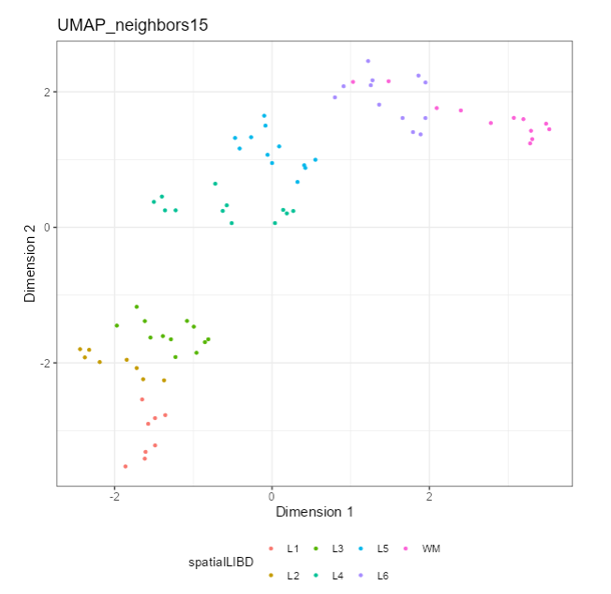
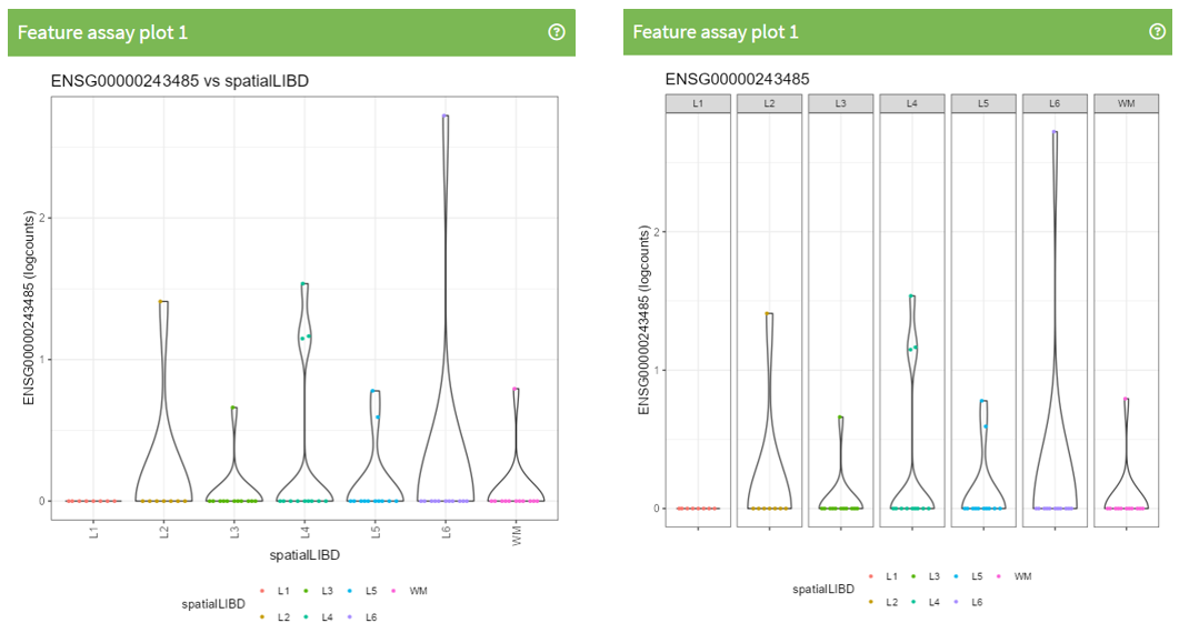
<p class="exercise">
**Question 1**:
 Which panel Type is displaying the following plot?
</p>

![](https://raw.githubusercontent.com/lcolladotor/cshl_rstats_genome_scale_2024/devel/Figures/iSEE_01_02.PNG)

<p class="exercise">
**Exercise 1**:
 Recreate the following plot.
</p>

![](https://raw.githubusercontent.com/lcolladotor/cshl_rstats_genome_scale_2024/devel/Figures/iSEE_01_02.PNG)

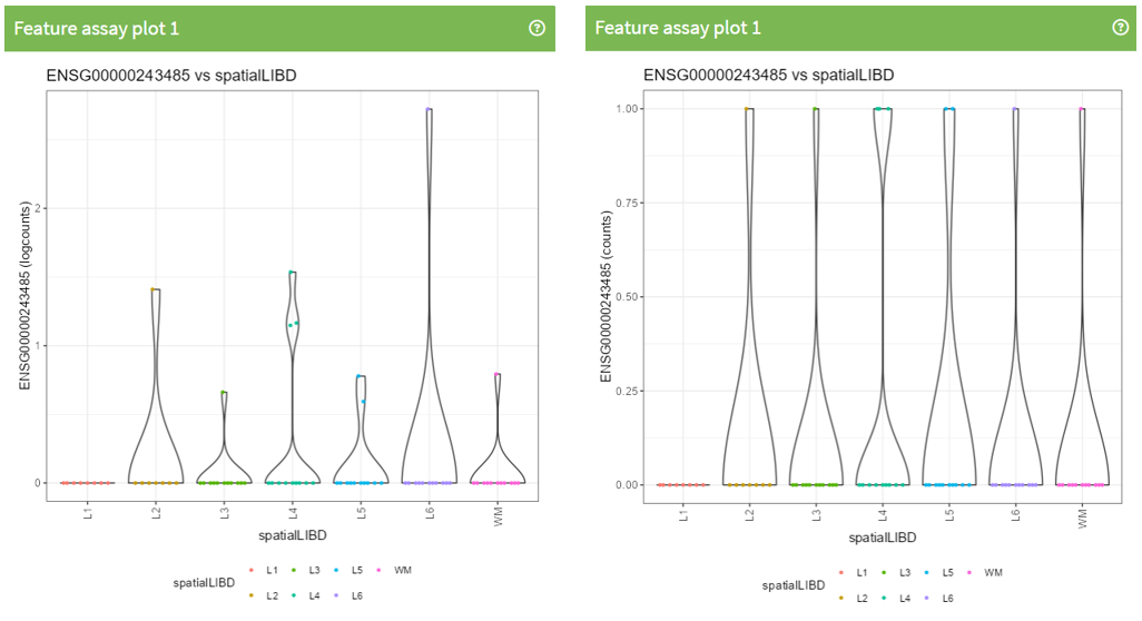
<p class="exercise">
**Question 2**:
 What is different between this 2 plots?
</p>

![](https://raw.githubusercontent.com/lcolladotor/cshl_rstats_genome_scale_2024/devel/Figures/iSEE_03.PNG)

<p class="exercise">
**Exercise 2**:
 Recreate the following plot.
</p>

![](https://raw.githubusercontent.com/lcolladotor/cshl_rstats_genome_scale_2024/devel/Figures/iSEE_04.PNG)

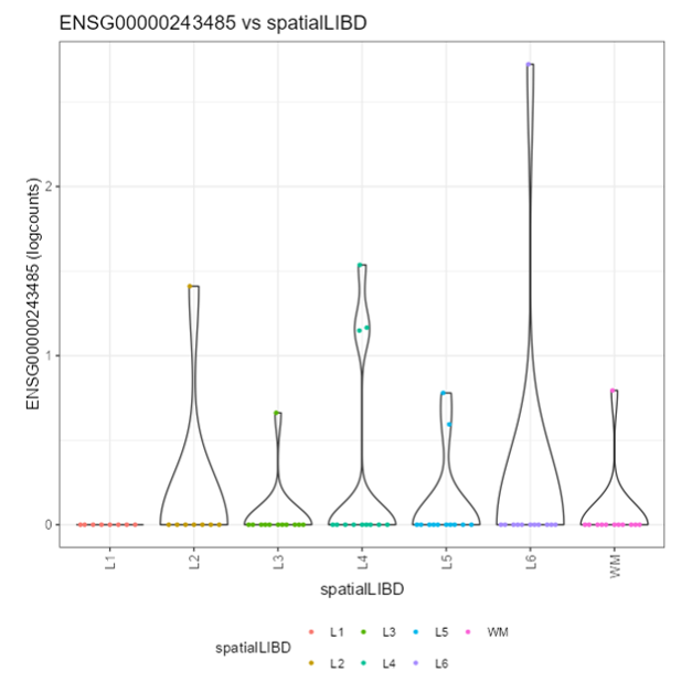
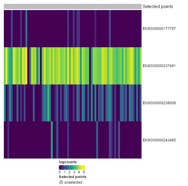
<p class="exercise">
**Question 3**:
 What is different between this 2 plots?
</p>

![](https://raw.githubusercontent.com/lcolladotor/cshl_rstats_genome_scale_2024/devel/Figures/iSEE_05.PNG)

<p class="exercise">
**Exercise 3**:
 Recreate the following plot
</p>

Ensembl IDs:
    ENSG00000177757
    ENSG00000237491
    ENSG00000238009
    ENSG00000243485

![](https://raw.githubusercontent.com/lcolladotor/cshl_rstats_genome_scale_2024/devel/Figures/iSEE_06.PNG)

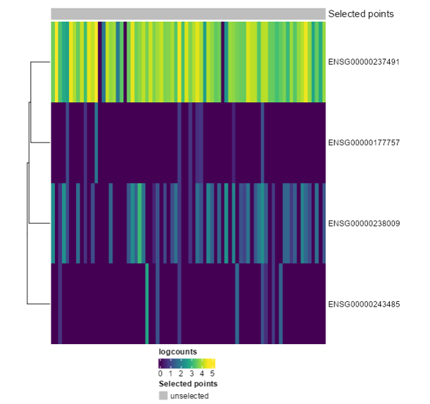
<p class="exercise">
**Exercise 4**:
 Recreate the following plot. What would you change from the last one?
</p>

Ensembl IDs:
    ENSG00000177757
    ENSG00000237491
    ENSG00000238009
    ENSG00000243485

![](https://raw.githubusercontent.com/lcolladotor/cshl_rstats_genome_scale_2024/devel/Figures/iSEE_07.PNG)

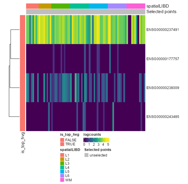
<p class="exercise">
**Exercise 5**:
 Recreate the following plot. What would you change from the last one?
</p>

Ensembl IDs:
    ENSG00000177757
    ENSG00000237491
    ENSG00000238009
    ENSG00000243485

![](https://raw.githubusercontent.com/lcolladotor/cshl_rstats_genome_scale_2024/devel/Figures/iSEE_08.PNG)

<p class="exercise">
**Exercise 6**:
 Download only the last plot (Final HeatMap)
</p>

<p class="exercise">
**Exercise 7**:
 Extract the R code only for the last plot(Final HeatMap)
</p>


## Introduction to Advanced iSEE Features

Adapted from the GitHub Issue: https://github.com/iSEE/iSEE/issues/650

Beyond its basic functionalities, `iSEE` offers advanced features that allow users to perform complex data manipulations interactively. This includes the ability to subset and filter cells based on gene expression criteria.

To begin with, we will load the necessary libraries and dataset. In this case we will be using `ReprocessedAllenData` from the `scRNAseq` package, a dataset of 379 mouse brain cells from Tasic et al. (2016).
After loading the dataset, we normalize the counts and perform a PCA (Principal Component Analysis) to prepare the data for visualization. 

```{r, load_scRNAseq_data}
library("scRNAseq")
library("scater")
library("iSEE")

# Load the dataset
sce <- ReprocessedAllenData(assays = "tophat_counts")

# Normalize counts and perform PCA
sce <- logNormCounts(sce, exprs_values = "tophat_counts")
sce <- runPCA(sce, ncomponents = 4)
```

### Selecting Cells Based on a Single Gene Expression

To select cells based on the expression of a single gene using iSEE, we need to *create an initial list of panels that will be displayed when we launch iSEE*. The first panel in our list is a "FeatureAssayPlot", which will show the expression levels of the gene "Serpine2". By visualizing this plot, we can interactively select cells that express "Serpine2".

To complement this, we add a "ReducedDimensionPlot" to our panel list. This plot will visualize the PCA and highlight the cells that we selected based on "Serpine2" expression. The linkage between these two panels allows us to see how the selected cells are distributed in the reduced dimensional space (PCA).

```{r, single_geneExpr}
## Initial settings for a single gene expression
initial_single <- list(
    FeatureAssayPlot(Assay = "logcounts", YAxisFeatureName = "Serpine2"),
    ReducedDimensionPlot(Type = "PCA", ColorBy = "Column selection", ColumnSelectionSource = "FeatureAssayPlot1")
)

## Launch iSEE with the initial settings
if (interactive()) {
    iSEE(sce, initial = initial_single)
}
```

### Using a Single Plot for Two Gene Co-Expression

To select cells based on the expression of two gene, we can use a single "FeatureAssayPlot" panel. In this setup, one gene is plotted on the x-axis and the other gene on the y-axis. This method allows us to directly visualize and select cells that express both genes simultaneously.

By adding a "ReducedDimensionPlot" to our initial panel list, we can again see how these selected cells are distributed in the PCA plot. This approach is simpler when dealing with only two genes and provides an intuitive way to explore co-expression patterns.

```{r, 2_genesExpr}
## Initial settings for 2 genes expression on the same "FeatureAssayPlot"
initial_combined <- list(
    FeatureAssayPlot(Assay = "logcounts", XAxis = "Feature name", XAxisFeatureName = "Serpine2", YAxisFeatureName = "Bcl6"),
    ReducedDimensionPlot(Type = "PCA", ColorBy = "Column selection", ColumnSelectionSource = "FeatureAssayPlot1")
)

## Launch iSEE with the initial settings
if (interactive()) {
    iSEE(sce, initial = initial_combined)
}
```

### Selecting Cells Based on the Co-Expression of Two or more Genes

In situations where we want to select cells based on the expression of two or more genes, we need to chain multiple "FeatureAssayPlot" panels together. For instance, if we are interested in cells that express both "Serpine2" and "Bcl6", we start by creating a "FeatureAssayPlot" for "Serpine2". Then, we add another "FeatureAssayPlot" for "Bcl6", but this time we specify that the selection source for this plot is the "FeatureAssayPlot" for "Serpine2". This setup ensures that only cells that were selected in the first plot (based on "Serpine2") are displayed in the second plot (for" Bcl6").

Finally, we include a ReducedDimensionPlot to visualize the PCA, highlighting the cells that meet both criteria. This chained selection process allows for more refined filtering based on multiple gene expressions.

```{r, chain_FeatureAssayPlots}
## Initial settings chainning multiple "FeatureAssayPlot"
initial_double <- list(
    FeatureAssayPlot(Assay = "logcounts", YAxisFeatureName = "Serpine2"),
    FeatureAssayPlot(Assay = "logcounts", YAxisFeatureName = "Bcl6", ColumnSelectionSource = "FeatureAssayPlot1", ColumnSelectionRestrict = TRUE),
    ReducedDimensionPlot(Type = "PCA", ColorBy = "Column selection", ColumnSelectionSource = "FeatureAssayPlot2")
)

## Launch iSEE with the initial settings
if (interactive()) {
    iSEE(sce, initial = initial_double)
}
```

## References

* https://www.bioconductor.org/packages/release/bioc/html/iSEE.html
* https://github.com/iSEE/iSEE
* https://shiny.posit.co/r/gallery/life-sciences/isee/
* https://bioconductor.org/packages/release/bioc/vignettes/iSEE/inst/doc/basic.html
* https://github.com/iSEE/iSEE/issues/650

## Community

`iSEE` authors:

* Kévin Rue-Albrecht https://twitter.com/KevinRUE67
* Federico Marini https://twitter.com/FedeBioinfo
* Charlotte Soneson https://bsky.app/profile/csoneson.bsky.social
* Aaron Lun https://twitter.com/realAaronLun