strand-seq-read-plots

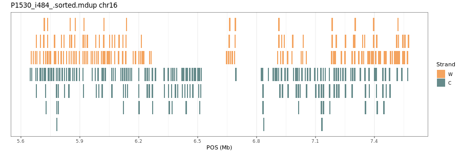
Workflow to plot the individual reads in a region of interest in a Strand-seq library. Written by Benedict March 2023, please let me know if you have any suggestions/issues!

0. Setup

Clone this repository like so:

git clone https://github.com/Sanders-Lab/strand-seq-read-plots

Then you can change directory into the created folder to run the scripts:

cd strand-seq-read-plots

For the shell script you will need samtools installed and in your environment (e.g. via conda: conda install -c bioconda samtools). For the R script you will require tidyverse for dplyr & ggplot2, which you can load with library(tidyverse) or install with install.packages("tidyverse"). Note that due to dependency issues, you may find it better to have samtools and R in different conda environments.

1. Extract reads

The first step is to execute 1_extract_reads.sh to extract the Watson and Crick reads:

bash 1_extract_reads.sh \
  /fast/groups/ag_sanders/work/data/strand_seq/internal/human/P1530/bam \
  chr16:5643516-7570129 \
  P1530_example_output.txt

Where the 1st command line argument is a directory containing the bam files of interest, the 2nd is the region of interest (format CHROM:Start-End), and the 3rd is a filepath for the output file.

2. Plot reads

Next you can plot the reads in your region of interest in R, by sourcing the plot_counts() function in 2_plot_reads.R. Here is an example script to visualise a region of interest on chr16 on P1530_i484:

source('2_plot_reads.R')
library(tidyverse)

reads_df = read.table("P1530_example_output.txt.gz", header = T) %>%
  filter(cell == "P1530_i484_.sorted.mdup")
  
png("P1530_chr16_example_plot.png", width = 900, height = 300)
plot_counts(input_df = reads_df)
dev.off()

The output is the graph below. Enjoy!