Dose influence matrix calculation
matRad's dose influence matrix calculation algorithms are split into two parts: First we determine the irradiation geometry by generating the steering information for the desired beam setup. In a second step, we generate dosimetric information by pre-computing dose influence matrices for inverse planning.
The steering information holds all geometric information about the irradiation within the stf struct. It is generated by calling matRad_generateStf.
The stf struct uses both the LPS coordinate system and a beam's eye view coordinate system in [mm]. Coordinates in beam's eye view coordinate system are labeled accordingly; coordinates in LPS coordinate system do not have an extra label.
The irradiation geometry is organized to a ray and bixel concept, which is schematically shown below.
Schematic visualization of the ray and bixel concept
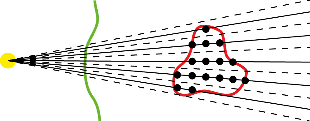
From a virtual radiation source (yellow) the target volume (red) within the patient (green) is covered by equidistant rays (solid black). Note that only a two-dimensional cut through a three dimensional cone of rays is shown for clarity. In the isocenter plane (not shown) the distance of the individual rays corresponds to the bixel width (compare pln struct). For photons, the term bixel refers to a discrete rectangular fluence element (the limits of the individual bixels are shown in dashed black). Together, all bixels cover the entire target volume.
For 3D IMPT for particles, we have an additional degree of freedom, namely the particle energy to be considered. This is accounted for during the stf-struct generation by determining the depth of the target volume on individual rays and placing spots (black dots) accordingly.
More information about the ray and bixel concept (though with slight variations in nomenclature) can be found in sections 2.3 and 2.5 Nill (2001).
Based on the steering information, matRad can compute dose for individual photon bixels or proton/carbon ion pencil beams. The required geometric and radiological distances facilitate the same set of matRad functions.
We perform an exact calculation of the radiological depth for the entire irradiated volume with a ray tracing algorithm in matRad_rayTracing according to Siddon (1985) Medical Physics and Siggel (2012) Physica Medica.
Geometric distances from the lateral distances to the central ray are computed by standard matrix vector algebra in matRad_calcRadGeoDists.
matRad uses a singular value decomposed pencil beam algorithm implemented according to Bortfeld et al. (1993) Medical Physics. The functionalities are organized in the matRad functions matRad_calcPhotonDose and matRad_calcPhotonDoseBixel. A more detailed description of the inner workings of the algorithm can also be found in the diploma thesis of Martin Siggel "Entwicklung einer schnellen Dosisberechnung auf Basis eines Pencil-Kernel Algorithmus für die Strahlentherapie mit Photonen" (Universität Heidelberg, 2008) which is available for download here.
The dose delivered to a certain voxel i from bixel j is stored as dose influence matrix in the dij struct using MATLAB's built-in double precision sparse matrix format.
The necessary measured base data, namely the kernel functions as described by Bortfeld et al. (1993) Medical Physics are supplied for a 6MV LINAC and stored in photons_Generic.mat as MATLAB piecewise polynomial.
matRad's photon dose engine is calibrated such that a bixel intensity of all ones, i.e., w = ones(stf.totalNumOfBixels,1), yields a dose of roughly 1Gy in 5cm depth for a 5cm by 5cm field at SSD = 900mm. If you want to reproduce this, you can download a set of stf and pln structures that work with the TG119 phantom here.
For the photon dose calculation, we assume a uniform primary fluence. While this should not have any impact on the resulting dose distributions, as we allow for intensity-modulation, this reduces the computation time because we only have to perform one convolution and we can compute the individual contributions from different bixels with the same kernel matrices (kernel1Mx, kernel2Mx, kernel3Mx). An extension to inhomogeneous primary fluences is easily possible.
To model a virtual photon source with finite size, the primary fluence is convolved with a Gaussian filter. The size of this filter is determined by the measured penumbra at isocenter, which is related to the source size as depicted in the following images from Martin Siggel's (Siggel M. Entwicklung einer schnellen Dosisberechnung auf Basis eines Pencil-Kernel Algorithmus für die Strahlentherapie mit Photonen. Diploma Thesis 2008, Universität Heidelberg):


matRad initially used a hardcoded value of 5mm for the measured penumbra with. From version 2.10.1 on, the value can also be stored in the photon base data file so that it can also be translated to the virtual source size for, for example, Monte Carlo simulations.
For the photon dose calculation, there are three main possibilities to speed up computations and reduce memory consumption.
- It is possible to reduce the spatial resolution of the dose calculation in the patient CT by downsampling the CT data upon import. If you do this as a post-processing step, be aware you need to adjust the binary segmentations in the cst cell array accordingly.
- You can increase the variable pln.bixelWidth in the matRad script which effectively reduces the number of bixels which have to be computed approximately quadratically.
- You can reduce the radius around the central ray, around which dose is computed by adjusting the variable lateralCutOff in matRad_calcPhotonDose. Currently this variable is already set to 50mm.
matRad facilitates a conventional pencil beam model for particle dose calculations similar to the work of Hong et al. (1996). The dose at a particular voxel is given as the product of a depth dependent part and a lateral part. For the depth dependent part, matRad uses tabulated depth dose curves for individual particle energies. For lateral beam broadening, matRad uses a depth-dependent sigma of a Gaussian profile, which is also tabulated versus depth for all available beam energies.
The dose delivered to a certain voxel i from bixel j is stored as dose influence matrix in the dij struct using MATLAB's built-in double precision sparse matrix format.
For carbon ions, matRad also enables the computation of α- and β-matrices that can be used to compute three-dimensional dose weighted α- and β-distributions, which can in turn be used to compute three-dimensional RBE distributions during inverse planning.
matRad only models variations of α and β with depth in matRad_calcLQParameter. Potential dependencies in lateral direction are not explicitly modeled.
The base data files protons_Generic and carbon_Generic required for particle dose calculation include depth dose curves and tabulated lateral beam widths (as Gaussian sigmas) for a library of different energies. The proton base data has been computed based on an analytical approximation for the Bragg curve (Bortfeld (1997)) and Highland's approximation for multiple Coulomb scattering (Gottschalk (1993)). The carbon ion base data has been Monte Carlo simulated for an idealized beam line without monitoring devices. Besides this physical information, the carbon ion base data also includes α and β tables that have been computed based on LEM IV. Within the *.mat files, the depth is stored in [mm], α tables are stored in [1/Gy], β tables are stored in [1/Gy^2], and the integrated depth dose distribution is stored in [MeV cm^2 /(g * primary)]. Upon dose calculation, the integrated depth dose is converted to [Gy mm^2 /(1e6 primaries)] with a linear scaling in the function matRad_calcParticleDoseBixel.m. Given that the lateral components of the dose calculation have the unit [1/mm^2], the weight of the pencil beams in matRad directly corresponds to the number of particles in [1e6] while the dose is given in [Gy].
More detailed information on the structure of a particle base data file is given here!
Besides the standard approximations made by pencil beam algorithms (i.e. factorization of lateral and depth-dependent part, ray tracing only on central ray), we do not make any approximations for particle dose calculation.
For the particle dose calculation, there are three main possibilities to speed up computations and reduce memory consumption.
- It is possible to reduce the spatial resolution of the dose calculation in the patient CT by downsampling the CT data upon import. If you do this as a post-processing step, be aware you need to adjust the binary segmentations in the cst cell array accordingly.
- You can increase the variable
pln.propStf.bixelWidthin the matRad script which effectively reduces the number of pencil beams which have to be computed approximately quadratically. - You can reduce the radius around the central ray where dose is computed by adjusting the variable lateralCutOff in matRad_calcParticleDose.
| Home | About |
Quick Setup |
Technical Docs | FAQ |