NOTE! This is my personal note from the Kaggle course, and related sources. Before this course Highly recommend Computer Aided Solution Processing and Artificial Intelligence - Intelligent agents paradigm courses.
Use TensorFlow and Keras to build and train neural networks for structured data.
The Course was written by Ryan Holbrook and Builds on Intro to Machine Learning Kaggle course. You can find my notes about that here.
file:exercise-a-single-neuron.ipynb
Some of the most impressive advances in artificial intelligence in recent years have been in the field of deep learning. Natural language translation, image recognition, and game playing are all tasks where deep learning models have neared or even exceeded human-level performance.
So what is deep learning? Deep learning is an approach to machine learning characterized by deep stacks of computations. This depth of computation is what has enabled deep learning models to disentangle the kinds of complex and hierarchical patterns found in the most challenging real-world datasets.
Through their power and scalability neural networks have become the defining model of deep learning. Neural networks are composed of neurons, where each neuron individually performs only a simple computation. The power of a neural network comes instead from the complexity of the connections these neurons can form.
So let's begin with the fundamental component of a neural network: the individual neuron. As a diagram, a neuron (or unit) with one input looks like:
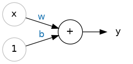
The Linear Unit:
Though individual neurons will usually only function as part of a larger network, it's often useful to start with a single neuron model as a baseline. Single neuron models are linear models.
Based on the 80 Cereals dataset we could estimate the calorie content of a cereal with 5 grams of sugar per serving like this:
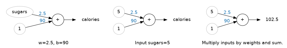
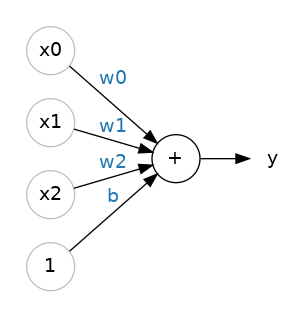
What if we wanted to expand our model to include things like fiber or protein content? That's easy enough. We can just add more input connections to the neuron, one for each additional feature. To find the output, we would multiply each input to its connection weight and then add them all together.
The formula for this neuron would be
Linear Units in Keras
"Keras is an API designed for human beings, not machines. Keras follows best practices for reducing cognitive load: it offers consistent & simple APIs, it minimizes the number of user actions required for common use cases, and it provides clear & actionable error messages. Keras also gives the highest priority to crafting great documentation and developer guides."
The easiest way to create a model in Keras is through keras.Sequential, which creates a neural network as a stack of layers. We can create models like those above using a dense layer (which we'll learn more about in the next lesson).
We could define a linear model accepting three input features ('sugars', 'fiber', and 'protein') and producing a single output ('calories') like so:
from tensorflow import keras
from tensorflow.keras import layers

# Create a network with 1 linear unit
model = keras.Sequential([
    layers.Dense(units=1,         # define how many outputs we want.
                 input_shape=[3]) # we tell Keras the dimensions of the inputs. Setting input_shape=[3] ensures the model will accept three features as input ('sugars', 'fiber', and 'protein').
])
The data we'll use in this course will be tabular data, like in a Pandas dataframe. We'll have one input for each feature in the dataset. The features are arranged by column, so we'll always have
input_shape=[num_columns]. The reason Keras uses a list here is to permit use of more complex datasets. Image data, for instance, might need three dimensions:[height, width, channels].Internally, Keras represents the weights of a neural network with tensors. Tensors are basically TensorFlow's version of a Numpy array with a few differences that make them better suited to deep learning. One of the most important is that tensors are compatible with GPU and TPU) accelerators. TPUs, in fact, are designed specifically for tensor computations.
A model's weights are kept in its
weightsattribute as a list of tensors. Get the weights of the model you defined above. (If you want, you could display the weights with something like:print("Weights\n{}\n\nBias\n{}".format(w, b))).
You can get the used weights like this:
w, b = model.weights
print("Weights\n{}\n\nBias\n{}".format(w, b))
Keras represents weights as tensors, but also uses tensors to represent data. When you set the input_shape argument, you are telling Keras the dimensions of the array it should expect for each example in the training data. Setting input_shape=[3] would create a network accepting vectors of length 3, like [0.2, 0.4, 0.6].
The key idea here is modularity, building up a complex network from simpler functional units. We've seen how a linear unit computes a linear function -- now we'll see how to combine and modify these single units to model more complex relationships.

A dense layer of two linear units receiving two inputs and a bias.
Neural networks typically organize their neurons into layers. When we collect together linear units having a common set of inputs we get a dense layer.
You could think of each layer in a neural network as performing some kind of relatively simple transformation. Through a deep stack of layers, a neural network can transform its inputs in more and more complex ways. In a well-trained neural network, each layer is a transformation getting us a little bit closer to a solution.
A "layer" in Keras is a very general kind of thing. A layer can be, essentially, any kind of data transformation. Many layers, like the convolutional and recurrent layers, transform data through use of neurons and differ primarily in the pattern of connections they form. Others though are used for feature engineering or just simple arithmetic. There's a whole world of layers to discover!
more:
It turns out, however, that two dense layers with nothing in between are no better than a single dense layer by itself. Dense layers by themselves can never move us out of the world of lines and planes. What we need is something nonlinear. What we need are activation functions. An activation function is simply some function we apply to each of a layer's outputs (its activations). The most common is the rectifier function
 |
 |
|---|---|
| Without activation functions, neural networks can only learn linear relationships. In order to fit curves, we'll need to use activation functions. | The Rectifier Function |
The rectifier function has a graph that's a line with the negative part "rectified" to zero. Applying the function to the outputs of a neuron will put a bend in the data, moving us away from simple lines.
When we attach the rectifier to a linear unit, we get a rectified linear unit or ReLU. (For this reason, it's common to call the rectifier function the "ReLU function".) Applying a ReLU activation to a linear unit means the output becomes max(0, w * x + b), which we might draw in a diagram like:
A rectified linear unit.
Now that we have some nonlinearity, let's see how we can stack layers to get complex data transformations.

A stack of dense layers makes a "fully-connected" network.
The layers before the output layer are sometimes called hidden since we never see their outputs directly. Now, notice that the final (output) layer is a linear unit (meaning, no activation function). That makes this network appropriate to a regression task, where we are trying to predict some arbitrary numeric value. Other tasks (like classification) might require an activation function on the output. Remember, Classification is the task of predicting a discrete class label. Regression is the task of predicting a continuous quantity. h2o.ai
The Sequential model we've been using will connect together a list of layers in order from first to last: the first layer gets the input, the last layer produces the output. This creates the model in the figure above. Be sure to pass all the layers together in a list, like [layer, layer, layer, ...], instead of as separate arguments. To add an activation function to a layer, just give its name in the activation argument. More about sequential models
from tensorflow import keras
from tensorflow.keras import layers

model = keras.Sequential([
    # the hidden ReLU layers
    layers.Dense(units=4, activation='relu', input_shape=[2]),
    layers.Dense(units=3, activation='relu'),
    # the linear output layer
    layers.Dense(units=1),
])file:exercise-stochastic-gradient-descent.ipynb
As with all machine learning tasks, we begin with a set of training data. Each example in the training data consists of some features (the inputs) together with an expected target (the output). Training the network means adjusting its weights in such a way that it can transform the features into the target. In the 80 Cereals dataset, for instance, we want a network that can take each cereal's
'sugar','fiber', and'protein'content and produce a prediction for that cereal's'calories'. If we can successfully train a network to do that, its weights must represent in some way the relationship between those features and that target as expressed in the training data.In addition to the training data, we need two more things
- A "loss function" that measures how good the network's predictions are.
- An "optimizer" that can tell the network how to change its weights.
We've seen how to design an architecture for a network, but we haven't seen how to tell a network what problem to solve. This is the job of the loss function.
The loss function measures the disparity between the the target's true value and the value the model predicts.
Different problems call for different loss functions. We have been looking at regression problems, where the task is to predict some numerical value -- calories in 80 Cereals, rating in Red Wine Quality. Other regression tasks might be predicting the price of a house or the fuel efficiency of a car.
A common loss function for regression problems is the mean absolute error or MAE. For each prediction y_pred, MAE measures the disparity from the true target y_true by an absolute difference abs(y_true - y_pred).
The total MAE loss on a dataset is the mean of all these absolute differences.
Where Where: n = the number of errors; |xi – x| = the absolute errors.

The mean absolute error is the average length between the fitted curve and the data points.
Besides MAE, other loss functions you might see for regression problems are the mean-squared error (MSE) or the Huber loss (both available in Keras).
During training, the model will use the loss function as a guide for finding the correct values of its weights (lower loss is better). In other words, the loss function tells the network its objective. The Optimizer - Stochastic Gradient Descent
We've described the problem we want the network to solve, but now we need to say how to solve it. This is the job of the optimizer. The optimizer is an algorithm that adjusts the weights to minimize the loss.
Virtually all of the optimization algorithms used in deep learning belong to a family called stochastic gradient descent. They are iterative algorithms that train a network in steps. One step of training goes like this:
- Sample some training data and run it through the network to make predictions.
- Measure the loss between the predictions and the true values
- Finally, adjust the weights in a direction that makes the loss smaller.
Then just do this over and over until the loss is as small as you like (or until it won't decrease any further.)

Training a neural network with Stochastic Gradient Descent (SGD).
Each iteration's sample of training data is called a minibatch (or often just "batch"), while a complete round of the training data is called an epoch. The number of epochs you train for is how many times the network will see each training example.
The animation shows the linear model from Lesson 1 being trained with SGD. The pale red dots depict the entire training set, while the solid red dots are the minibatches. Every time SGD sees a new minibatch, it will shift the weights (w the slope and b the y-intercept) toward their correct values on that batch. Batch after batch, the line eventually converges to its best fit. You can see that the loss gets smaller as the weights get closer to their true values.
Notice that the line only makes a small shift in the direction of each batch (instead of moving all the way). The size of these shifts is determined by the learning rate. A smaller learning rate means the network needs to see more minibatches before its weights converge to their best values.
The learning rate and the size of the minibatches are the two parameters that have the largest effect on how the SGD training proceeds. Their interaction is often subtle and the right choice for these parameters isn't always obvious. (We'll explore these effects in the exercise.)
Fortunately, for most work it won't be necessary to do an extensive hyperparameter search to get satisfactory results. Adam is an SGD algorithm that has an adaptive learning rate that makes it suitable for most problems without any parameter tuning (it is "self tuning", in a sense). Adam is a great general-purpose optimizer.
After defining a model, you can add a loss function and optimizer with the model's compile method:
model.compile(
    optimizer="adam",
    loss="mae",
)
Notice that we are able to specify the loss and optimizer with just a string. You can also access these directly through the Keras API -- if you wanted to tune parameters, for instance -- but for us, the defaults will work fine.
What's In a Name?
The gradient is a vector that tells us in what direction the weights need to go. More precisely, it tells us how to change the weights to make the loss change fastest. We call our process gradient descent because it uses the gradient to descend the loss curve towards a minimum. Stochastic means "determined by chance." Our training is stochastic because the minibatches are random samples from the dataset. And that's why it's called SGD!