ILU for SparseMatrixCSC

This package implements the left-looking or Crout version of ILU for the SparseMatrixCSC type. It exports the function ilu.

How to install

IncompleteLU can be installed through the Julia package manager:

julia> ]
pkg> add IncompleteLU

The package is then available via

julia> using IncompleteLU

When to use this package

Whenever you need an incomplete factorization of a sparse and non-symmetric matrix.

The package also provides means to apply the factorization in-place via ldiv!, forward_substitution! and backward_substitution!. This is useful in the context of left, right or split preconditioning. See the example below.

Example

Using a drop tolerance of 0.01, we get a reasonable preconditioner with a bit of fill-in.

> using IncompleteLU, LinearAlgebra, SparseArrays
> using BenchmarkTools
> A = sprand(1000, 1000, 5 / 1000) + 10I
> fact = @btime ilu($A, τ = 0.001)
  2.894 ms (90 allocations: 1.18 MiB)
> norm((fact.L + I) * fact.U' - A)
0.05736313452207798
> nnz(fact) / nnz(A)
3.6793806030969844

Full LU is obtained when the drop tolerance is 0.0.

> fact = @btime ilu($A, τ = 0.)
  209.293 ms (106 allocations: 12.18 MiB)
> norm((fact.L + I) * fact.U' - A)
1.5262736852530086e-13
> nnz(fact) / nnz(A)
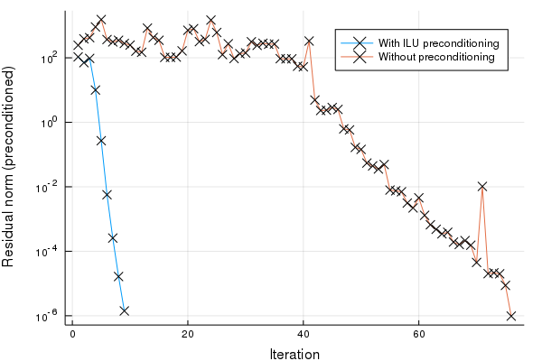
69.34213528932355

Preconditioner

ILU is typically used as preconditioner for iterative methods. For instance

using IterativeSolvers, IncompleteLU
using SparseArrays, LinearAlgebra
using BenchmarkTools
using Plots

"""
Benchmarks a non-symmetric n × n × n problem
with and without the ILU preconditioner.
"""
function mytest(n = 64)
    N = n^3

    A = spdiagm(
      -1 => fill(-1.0, n - 1), 
       0 => fill(3.0, n), 
       1 => fill(-2.0, n - 1)
    )
    Id = sparse(1.0I, n, n)
    A = kron(A, Id) + kron(Id, A)
    A = kron(A, Id) + kron(Id, A)
    x = ones(N)
    b = A * x

    LU = ilu(A, τ = 0.1)
    @show nnz(LU) / nnz(A)

    # Benchmarks
    prec = @benchmark ilu($A, τ = 0.1)
    @show prec
    with = @benchmark bicgstabl($A, $b, 2, Pl = $LU, max_mv_products = 2000)
    @show with
    without = @benchmark bicgstabl($A, $b, 2, max_mv_products = 2000)
    @show without

    # Result
    x_with, hist_with = bicgstabl(A, b, 2, Pl = LU, max_mv_products = 2000, log = true)
    x_without, hist_without = bicgstabl(A, b, 2, max_mv_products = 2000, log = true)

    @show norm(b - A * x_with) / norm(b) 
    @show norm(b - A * x_without) / norm(b)

    plot(hist_with[:resnorm], yscale = :log10, label = "With ILU preconditioning", xlabel = "Iteration", ylabel = "Residual norm (preconditioned)", mark = :x)
    plot!(hist_without[:resnorm], label = "Without preconditioning", mark = :x)
end

mytest()

Outputs

nnz(LU) / nnz(A) = 2.1180353639352374
prec = Trial(443.781 ms)
with = Trial(766.141 ms)
without = Trial(2.595 s)
norm(b - A * x_with) / norm(b) = 2.619046427010899e-9
norm(b - A * x_without) / norm(b) = 1.2501603557459283e-8

The algorithm

The basic algorithm loops roughly as follows:

for k = 1 : n
  row = zeros(n); row[k:n] = A[k,k:n]
  col = zeros(n); col[k+1:n] = A[k+1:n,k]

  for i = 1 : k - 1 where L[k,i] != 0
    row -= L[k,i] * U[i,k:n]
  end

  for i = 1 : k - 1 where U[i,k] != 0
    col -= U[i,k] * L[k+1:n,i]
  end

  # Apply a dropping rule in row and col

  U[k,:] = row
  L[:,k] = col / U[k,k]
  L[k,k] = 1
end

which means that at each step k a complete row and column are computed based on the previous rows and columns:

          k
+---+---+---+---+---+---+---+---+
| \ |   | x | x | x | x | x | x |
+---+---+---+---+---+---+---+---+
|   | \ | x | x | x | x | x | x |
+---+---+---+---+---+---+---+---+
|   |   | . | . | . | . | . | . | k
+---+---+---+---+---+---+---+---+
| x | x | . | \ |   |   |   |   |
+---+---+---+---+---+---+---+---+
| x | x | . |   | \ |   |   |   |
+---+---+---+---+---+---+---+---+
| x | x | . |   |   | \ |   |   |
+---+---+---+---+---+---+---+---+
| x | x | . |   |   |   | \ |   |
+---+---+---+---+---+---+---+---+
| x | x | . |   |   |   |   | \ |
+---+---+---+---+---+---+---+---+

col and row are the .'s, updated by the x's.

At step k we load (part of) a row and column of the matrix A, and subtract the previous rows and columns times a scalar (basically a SpMV product). The problem is that our matrix is column-major, so that loading a row is not cheap. Secondly, it makes sense to store the L factor column-wise and the U factor row-wise (so that we can append columns and rows without data movement), yet we need access to a row of L and a column of U.

The latter problem can be worked around without expensive searches. It's basically smart bookkeeping: going from step k to k+1 requires updating indices to the next nonzero of each row of U after column k. If you now store for each column of U a list of nonzero indices, this is the moment you can update it. Similarly for the L factor.

The matrix A can be read row by row as well with the same trick.

Accumulating a new sparse row or column

Throughout the steps two temporary row and column accumulators are used to store the linear combinations of previous sparse rows and columns. There are two implementations of this accumulator: the SparseVectorAccumulator performs insertion in O(1), but stores the indices unordered; therefore a sort is required when appending to the SparseMatrixCSC. The InsertableSparseVector performs insertion sort, which can be slow, but turns out to be fast in practice. The latter is a result of insertion itself being an O(1) operation due to a linked list structure, and the fact that sorted vectors are added, so that the linear scan does not have to restart at each insertion.

The advantage of SparseVectorAccumulator over InsertableSparseVector is that the former postpones sorting until after dropping, while InsertableSparseVector also performs insertion sort on dropped values.

Todo

The method does not implement scaling techniques, so the τ parameter is really an absolute dropping tolerance parameter.