Previously you've evaluated a multiple linear regression model by calculating metrics based on the fit of the training data. In this lesson you'll learn why it's important to split your data in a train and a test set if you want to evaluate a model used for prediction.
You will be able to:
- Perform a train-test split
- Prepare training and testing data for modeling
- Compare training and testing errors to determine if model is over or underfitting
Recall some ways that we can evaluate linear regression models.
It is pretty straightforward that, to evaluate the model, you'll want to compare your predicted values,
To get a summarized measure over all the instances, a popular metric is the (Root) Mean Squared Error:
RMSE =
MSE =
Larger (R)MSE indicates a worse model fit.
So far we've simply been fitting models to data, and evaluated our models calculating the errors between our
Let's say we want to predict the outcome for observations that are not necessarily in our dataset now; e.g: we want to predict miles per gallon for a new car that isn't part of our dataset, or predict the price for a new house in Ames.
In order to get a good sense of how well your model will be doing on new instances, you'll have to perform a so-called "train-test-split". What you'll be doing here, is taking a sample of the data that serves as input to "train" our model - fit a linear regression and compute the parameter estimates for our variables, and then calculate how well our predictive performance is doing based solely on the "test" data, comparing the actual targets
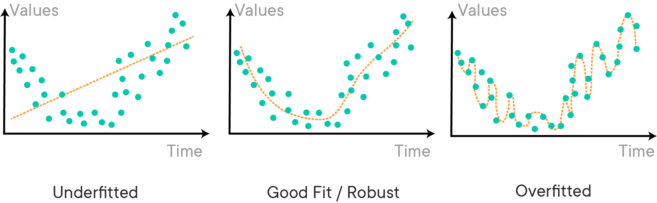
Another reason to use train-test-split is because of a common problem which doesn't only affect linear models, but nearly all (other) machine learning algorithms: overfitting and underfitting. An overfit model is not generalizable and will not hold to future cases. An underfit model does not make full use of the information available and produces weaker predictions than is feasible. The following image gives a nice, more general demonstration:
When performing a train-test-split, it is important that the data is randomly split. At some point, you will encounter datasets that have certain characteristics that are only present in certain segments of the data. For example, if you were looking at sales data for a website, you might expect the data to look different on days that promotional deals were held versus days that deals were not held. If we don't randomly split the data, there is a chance we might overfit to the characteristics of certain segments of data.
Another thing to consider is just how big each training and testing set should be. There is no hard and fast rule for deciding the correct size, but the range of training set is usually anywhere from 66% - 80% (and testing set between 33% and 20%). Some types of machine learning models need a substantial amount of data to train on, and as such, the training sets should be larger. Some models with many different tuning parameters will need to be validated with larger sets (the test size should be larger) to determine what the optimal parameters should be. When in doubt, just stick with training set sizes around 70% and test set sizes around 30%.
You could write your own pandas code to shuffle and split your data, but we'll use the convenient train_test_split function from scikit-learn instead. We'll also use the Auto MPG dataset.
import pandas as pd

data = pd.read_csv('auto-mpg.csv')
data.head().dataframe tbody tr th {
vertical-align: top;
}
.dataframe thead th {
text-align: right;
}
| mpg | cylinders | displacement | horsepower | weight | acceleration | model year | origin | car name | |
|---|---|---|---|---|---|---|---|---|---|
| 0 | 18.0 | 8 | 307.0 | 130 | 3504 | 12.0 | 70 | 1 | chevrolet chevelle malibu |
| 1 | 15.0 | 8 | 350.0 | 165 | 3693 | 11.5 | 70 | 1 | buick skylark 320 |
| 2 | 18.0 | 8 | 318.0 | 150 | 3436 | 11.0 | 70 | 1 | plymouth satellite |
| 3 | 16.0 | 8 | 304.0 | 150 | 3433 | 12.0 | 70 | 1 | amc rebel sst |
| 4 | 17.0 | 8 | 302.0 | 140 | 3449 | 10.5 | 70 | 1 | ford torino |
The train_test_split function (documentation here) takes in a series of array-like variables, as well as some optional arguments. It returns multiple arrays.
For example, this would be a valid way to use train_test_split:
from sklearn.model_selection import train_test_split

train, test = train_test_split(data)train.head().dataframe tbody tr th {
vertical-align: top;
}
.dataframe thead th {
text-align: right;
}
| mpg | cylinders | displacement | horsepower | weight | acceleration | model year | origin | car name | |
|---|---|---|---|---|---|---|---|---|---|
| 181 | 25.0 | 4 | 116.0 | 81 | 2220 | 16.9 | 76 | 2 | opel 1900 |
| 387 | 27.0 | 4 | 140.0 | 86 | 2790 | 15.6 | 82 | 1 | ford mustang gl |
| 381 | 38.0 | 6 | 262.0 | 85 | 3015 | 17.0 | 82 | 1 | oldsmobile cutlass ciera (diesel) |
| 308 | 38.1 | 4 | 89.0 | 60 | 1968 | 18.8 | 80 | 3 | toyota corolla tercel |
| 134 | 16.0 | 8 | 302.0 | 140 | 4141 | 14.0 | 74 | 1 | ford gran torino |
test.head().dataframe tbody tr th {
vertical-align: top;
}
.dataframe thead th {
text-align: right;
}
| mpg | cylinders | displacement | horsepower | weight | acceleration | model year | origin | car name | |
|---|---|---|---|---|---|---|---|---|---|
| 259 | 18.1 | 6 | 258.0 | 120 | 3410 | 15.1 | 78 | 1 | amc concord d/l |
| 300 | 34.5 | 4 | 105.0 | 70 | 2150 | 14.9 | 79 | 1 | plymouth horizon tc3 |
| 370 | 37.0 | 4 | 91.0 | 68 | 2025 | 18.2 | 82 | 3 | mazda glc custom l |
| 195 | 29.0 | 4 | 90.0 | 70 | 1937 | 14.2 | 76 | 2 | vw rabbit |
| 313 | 24.3 | 4 | 151.0 | 90 | 3003 | 20.1 | 80 | 1 | amc concord |
In this case, the DataFrame data was split into two DataFrames called train and test. train has 294 values (75% of the full dataset) and test has 98 values (25% of the full dataset). Note the randomized order of the index values on the left.
However you can also pass multiple array-like variables into train_test_split at once. For each variable that you pass in, you will get a train and a test copy back out.
Most commonly in this curriculum these are the inputs and outputs:
Inputs
Xy
Outputs
X_trainX_testy_trainy_test
y = data[['mpg']]
X = data.drop(['mpg', 'car name'], axis=1)

X_train, X_test, y_train, y_test = train_test_split(X, y)X_train.head().dataframe tbody tr th {
vertical-align: top;
}
.dataframe thead th {
text-align: right;
}
| cylinders | displacement | horsepower | weight | acceleration | model year | origin | |
|---|---|---|---|---|---|---|---|
| 90 | 8 | 400.0 | 150 | 4464 | 12.0 | 73 | 1 |
| 241 | 3 | 80.0 | 110 | 2720 | 13.5 | 77 | 3 |
| 3 | 8 | 304.0 | 150 | 3433 | 12.0 | 70 | 1 |
| 34 | 6 | 250.0 | 100 | 3329 | 15.5 | 71 | 1 |
| 45 | 4 | 140.0 | 72 | 2408 | 19.0 | 71 | 1 |
y_train.head().dataframe tbody tr th {
vertical-align: top;
}
.dataframe thead th {
text-align: right;
}
| mpg | |
|---|---|
| 90 | 13.0 |
| 241 | 21.5 |
| 3 | 16.0 |
| 34 | 17.0 |
| 45 | 22.0 |
We can view the lengths of the results like this:
print(len(X_train), len(X_test), len(y_train), len(y_test))294 98 294 98
However it is not recommended to pass in just the data to be split. This is because the randomization of the split means that you will get different results for X_train etc. every time you run the code. For reproducibility, it is always recommended that you specify a random_state, such as in this example:
X_train, X_test, y_train, y_test = train_test_split(X, y, random_state=42)Another optional argument is test_size, which makes it possible to choose the size of the test set and the training set instead of using the default 75% train/25% test proportions.
X_train, X_test, y_train, y_test = train_test_split(X, y, test_size=0.2, random_state=42)Note that the lengths of the resulting datasets will be different:
print(len(X_train), len(X_test), len(y_train), len(y_test))313 79 313 79
When using a train-test split, data preparation should happen after the split. This is to avoid data leakage. The general idea is that the treatment of the test data should be as similar as possible to how genuinely unknown data should be treated. And genuinely unknown data would not have been there at the time of fitting the scikit-learn transformers, just like it would not have been there at the time of fitting the model!
In some cases you will see all of the data being prepared together for expediency, but the best practice is to prepare it separately.
from sklearn.preprocessing import FunctionTransformer
import numpy as np

# Instantiate a custom transformer for log transformation
log_transformer = FunctionTransformer(np.log, validate=True)

# Columns to be log transformed
log_columns = ['displacement', 'horsepower', 'weight']

# New names for columns after transformation
new_log_columns = ['log_disp', 'log_hp', 'log_wt']

# Log transform the training columns and convert them into a DataFrame
X_train_log = pd.DataFrame(log_transformer.fit_transform(X_train[log_columns]),
                           columns=new_log_columns, index=X_train.index)

X_train_log.head().dataframe tbody tr th {
vertical-align: top;
}
.dataframe thead th {
text-align: right;
}
| log_disp | log_hp | log_wt | |
|---|---|---|---|
| 258 | 5.416100 | 4.700480 | 8.194229 |
| 182 | 4.941642 | 4.521789 | 7.852439 |
| 172 | 5.141664 | 4.574711 | 8.001020 |
| 63 | 5.762051 | 5.010635 | 8.327243 |
| 340 | 4.454347 | 4.158883 | 7.536364 |
# Log transform the test columns and convert them into a DataFrame
X_test_log = pd.DataFrame(log_transformer.transform(X_test[log_columns]),
                          columns=new_log_columns, index=X_test.index)

X_test_log.head().dataframe tbody tr th {
vertical-align: top;
}
.dataframe thead th {
text-align: right;
}
| log_disp | log_hp | log_wt | |
|---|---|---|---|
| 78 | 4.564348 | 4.234107 | 7.691200 |
| 274 | 4.795791 | 4.744932 | 7.935587 |
| 246 | 4.510860 | 4.094345 | 7.495542 |
| 55 | 4.510860 | 4.248495 | 7.578145 |
| 387 | 4.941642 | 4.454347 | 7.933797 |
from sklearn.preprocessing import OneHotEncoder

# Instantiate OneHotEncoder
# Need to use sparse_output=False for sklearn 1.2 or greater
ohe = OneHotEncoder(drop='first', sparse=False)

# Create X_cat which contains only the categorical variables
cat_columns = ['origin']
X_train_cat = X_train.loc[:, cat_columns]

# Transform training set
X_train_ohe = pd.DataFrame(ohe.fit_transform(X_train_cat),
                           index=X_train.index)
X_train_ohe.head().dataframe tbody tr th {
vertical-align: top;
}
.dataframe thead th {
text-align: right;
}
| 0 | 1 | |
|---|---|---|
| 258 | 0.0 | 0.0 |
| 182 | 0.0 | 0.0 |
| 172 | 0.0 | 0.0 |
| 63 | 0.0 | 0.0 |
| 340 | 0.0 | 0.0 |
# Drop transformed columns
cols_to_drop = log_columns + cat_columns
X_train = X_train.drop(columns=cols_to_drop)

# Combine the three datasets into training
X_train_tr = pd.concat([X_train, X_train_log, X_train_ohe], axis=1)
X_train_tr.head().dataframe tbody tr th {
vertical-align: top;
}
.dataframe thead th {
text-align: right;
}
| cylinders | acceleration | model year | log_disp | log_hp | log_wt | 0 | 1 | |
|---|---|---|---|---|---|---|---|---|
| 258 | 6 | 18.7 | 78 | 5.416100 | 4.700480 | 8.194229 | 0.0 | 0.0 |
| 182 | 4 | 14.9 | 76 | 4.941642 | 4.521789 | 7.852439 | 0.0 | 0.0 |
| 172 | 6 | 14.5 | 75 | 5.141664 | 4.574711 | 8.001020 | 0.0 | 0.0 |
| 63 | 8 | 13.5 | 72 | 5.762051 | 5.010635 | 8.327243 | 0.0 | 0.0 |
| 340 | 4 | 16.4 | 81 | 4.454347 | 4.158883 | 7.536364 | 0.0 | 0.0 |
# Transform testing set
X_test_ohe = pd.DataFrame(ohe.transform(X_test[cat_columns]),
                          index=X_test.index)
X_test_ohe.head().dataframe tbody tr th {
vertical-align: top;
}
.dataframe thead th {
text-align: right;
}
| 0 | 1 | |
|---|---|---|
| 78 | 1.0 | 0.0 |
| 274 | 1.0 | 0.0 |
| 246 | 0.0 | 1.0 |
| 55 | 0.0 | 0.0 |
| 387 | 0.0 | 0.0 |
X_test = X_test.drop(columns=cols_to_drop)

# Combine test set
X_test_tr = pd.concat([X_test, X_test_log, X_test_ohe], axis=1)
X_test_tr.head().dataframe tbody tr th {
vertical-align: top;
}
.dataframe thead th {
text-align: right;
}
| cylinders | acceleration | model year | log_disp | log_hp | log_wt | 0 | 1 | |
|---|---|---|---|---|---|---|---|---|
| 78 | 4 | 18.0 | 72 | 4.564348 | 4.234107 | 7.691200 | 1.0 | 0.0 |
| 274 | 4 | 15.7 | 78 | 4.795791 | 4.744932 | 7.935587 | 1.0 | 0.0 |
| 246 | 4 | 16.4 | 78 | 4.510860 | 4.094345 | 7.495542 | 0.0 | 1.0 |
| 55 | 4 | 20.5 | 71 | 4.510860 | 4.248495 | 7.578145 | 0.0 | 0.0 |
| 387 | 4 | 15.6 | 82 | 4.941642 | 4.454347 | 7.933797 | 0.0 | 0.0 |
Great, now that you have preprocessed all the columns, you can fit a linear regression model:
# convert feature names to strings so there is not a TypeError with sklearn

X_train_tr.columns = X_train_tr.columns.astype(str)
X_test_tr.columns = X_test_tr.columns.astype(str)
from sklearn.linear_model import LinearRegression
linreg = LinearRegression()
linreg.fit(X_train_tr, y_train)
y_hat_train = linreg.predict(X_train_tr)
y_hat_test = linreg.predict(X_test_tr)Look at the residuals and calculate the MSE for training and test sets:
train_residuals = y_hat_train - y_train
test_residuals = y_hat_test - y_test
mse_train = np.sum((y_train - y_hat_train)**2)/len(y_train)
mse_test = np.sum((y_test - y_hat_test)**2)/len(y_test)
print('Train Mean Squared Error:', mse_train)
print('Test Mean Squared Error:', mse_test)Train Mean Squared Error: mpg 9.091819
dtype: float64
Test Mean Squared Error: mpg 10.010059
dtype: float64
You can also do this directly using sklearn's mean_squared_error() function:
from sklearn.metrics import mean_squared_error

train_mse = mean_squared_error(y_train, y_hat_train)
test_mse = mean_squared_error(y_test, y_hat_test)
print('Train Mean Squared Error:', train_mse)
print('Test Mean Squared Error:', test_mse)
Train Mean Squared Error: 9.091818811315937
Test Mean Squared Error: 10.01005948400949
Great, there does not seem to be a big difference between the train and test MSE!
In other words, our evaluation process has indicated that we are not overfitting. In fact, we may be underfitting because linear regression is not a very complex model.
Just for the sake of example, here is a model that is overfit to the data. Don't worry about the model algorithm being shown! Instead, just look at the MSE for the train vs. test set, using the same preprocessed data:
from sklearn.tree import DecisionTreeRegressor

other_model = DecisionTreeRegressor(random_state=42)
other_model.fit(X_train_tr, y_train)

other_train_mse = mean_squared_error(y_train, other_model.predict(X_train_tr))
other_test_mse = mean_squared_error(y_test, other_model.predict(X_test_tr))
print('Train Mean Squared Error:', other_train_mse)
print('Test Mean Squared Error:', other_test_mse)
Train Mean Squared Error: 0.0
Test Mean Squared Error: 11.403164556962025
This model initially seems great...0 MSE for the training data! But then you see that it is performing worse than our linear regression model on the test data. This model is overfitting.
This blog post shows a walkthrough of the key steps for model validation with train-test split and scikit-learn.
In this lesson, you learned the importance of the train-test split approach and used one of the most popular metrics for evaluating regression models, (R)MSE. You also saw how to use the train_test_split function from sklearn to split your data into training and test sets, and then evaluated whether models were overfitting using metrics on those training and test sets.